We demonstrate how to compute interest rates of yearly payments with Euler.
>load interest
Computes interest rates for investments.
The basic function is rate(v), which computes the interest of a vector of yearly payments. Assume, you pay 100 to a bank at 5%. You get a return of 5 each year, and finally 105.
So the plan is [-100,5,5,5,105], where negative numbers are payments, and positive numbers are returns.
Let us check the rate of this investment plan. It should be 5%, of course.
>rate([-100,5,5,5,105])
5
If we leave the interest rates on the bank, we get more at the end. Assume, we get 140.
What is the interest rate? We print the result as % this time.
>rate([-100,0,0,0,140]); print(%,digits=2,unit="%")
8.78%
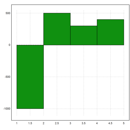
It is more interesting to solve irregular payments. E.g., assume we invest 1000, and get three returns 500, 300, and finally 400.
What would be the interest rate? It turns out to be approximately 10%.
>v:=[-1000,500,300,400]; P:=rate(v)
10.1789697676
Let us plot the payments.
>plot2d(v,bar=1):
We simulate this looping through the years. We assume a depth of 1000 and paybacks from the vector v, using the computed interest rate. Indeed the the final amount is 0.
>s:=0; for i=1 to length(v); s=s*(1+P/100)+v[i], end;
-1000
-601.789697676
-363.045689067
0
There is a function for this in interest.e.
>simrate(v,P)
[-1000, -601.79, -363.046, -2.27374e-013]
For more reality, we can add rounding to 2 digits.
>simrate(v,P,2)
[-1000, -601.79, -363.05, 0]
How does rate(v) work?
The function uses the Newton algorithm to solve for the interest rate. If we set x=1/(1+P/100) as the discount factor, we have to find the solution near 1 of a polynomial.
In the following test, we solve the polynomial using the secant method.
>x0:=solve("-1000+500*x+300*x^2+400*x^3",1)
0.907614222668
From x, we can compute P.
>(1/x0-1)*100
10.1789697676
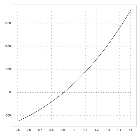
The Newton method works well for all plans, that have only one sign change. In this case the polynomial will be monotonically increasing.
>plot2d("-1000+500*x+300*x^2+400*x^3",0.5,1.5):
For the next example, we take a loan of 100'000, which we intend to pay back in 10 years with 10 rates of 5'000, beginning at the end of the first year after the loan. The final dept is 65'000. What is the interest rate?
We use the Euler matrix language to compute the vector of payments. Note that we have to pay the last rate plus the final amount after 10 years.
>v=100000|dup(-5000,9)'|-70000; plot2d(v,bar=1):
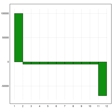
This loan has a very moderate interest rate.
>rate(v)
1.76978010371
How high would the final debt be, if the interest rate was 3%?
To compute this, we simulate the 10 payments at that interest rate. The last value is the final dept.
>simrate(100000|dup(-5000,10)',3,2)[-1]
77072.24
There is a function "investment", which solves all regular cases of loans or savings.
For a loan, we assume the start of the payments at the beginning of year 1, and stop at the beginning of year n. that is a total of n payments. The last two numbers indicate the start and the end.
>investment(100000,-5000,-65000,10,1,0)
1.7697801037
For a savings account, we start at the 0-th year, and end at year n-1. The account is computed for the end of the n-th year.
>investment(0,-1000,14500,10,0,1)
6.65746604866